Example: Estimating CATEs with a MetaLearner

Loading the data

First, we will load and prepare some data for this example. In this particular case we rely on the so-called mindset data set, taken from here and under MIT License. It stems from an experimental setup where

• The outcome was the achievement of a student in scalar form, found in column "achievement_score".

• The mindset intervention is a binary variable found in the column "intervention".

• Both numerical and categorical covariates/features are present.

import pandas as pd
from pathlib import Path
from git_root import git_root

df = pd.read_csv(git_root("data/learning_mindset.zip"))
outcome_column = "achievement_score"
treatment_column = "intervention"
feature_columns = [
    column
    for column in df.columns
    if column not in [outcome_column, treatment_column]
]
categorical_feature_columns = [
    "ethnicity",
    "gender",
    "frst_in_family",
    "school_urbanicity",
    "schoolid",
]
# Note that explicitly setting the dtype of these features to category
# allows both lightgbm as well as shap plots to
# 1. Operate on features which are not of type int, bool or float
# 2. Correctly interpret categoricals with int values to be
#    interpreted as categoricals, as compared to ordinals/numericals.
for categorical_feature_column in categorical_feature_columns:
    df[categorical_feature_column] = df[categorical_feature_column].astype(
        "category"
    )

Using a first, simple MetaLearner

Now that the data has been loaded, we can get to actually using MetaLearners. Let’s start with the TLearner. Investigating its documentation, we realize that only three initialization parameters are necessary in the case we do not want to reuse nuisance models: nuisance_model_factory, is_classification and n_variants. Given that our outcome is a scalar, we want to set is_classification=False and use a regressor as the nuisance_model_factory. In this case we arbitrarily choose a regressor from lightgbm. Since we know that the intervention was binary, we set n_variants=2.

from metalearners import TLearner
from lightgbm import LGBMRegressor

tlearner = TLearner(
    nuisance_model_factory=LGBMRegressor,
    is_classification=False,
    n_variants=2,
    nuisance_model_params={"verbose": -1}
)

Once our T-Learner has been instantiated, we can use it in a fashion akin to scikit-learn’s Estimator protocol. The subtle differences to aforementioned scikit-learn protocol are that

• We need to specify the observed treatment assignment w in the call to the fit method.

• We need to specify whether we want in-sample or out-of-sample CATE estimates in the predict() call via is_oos. In the case of in-sample predictions, the data passed to predict() must be exactly the same as the data that was used to call fit().

tlearner.fit(
    X=df[feature_columns],
    y=df[outcome_column],
    w=df[treatment_column],
)

cate_estimates_tlearner = tlearner.predict(
    X=df[feature_columns],
    is_oos=False,
)

We can now notice that cate_estimates_tlearner is of shape \((n_{obs}, n_{variants} - 1, n_{outputs})\). This is meant to cater to a general case, where there are more than two variants and/or classification problems with many class probabilities. Given that we care about the simple case of binary variant regression, we can make use of simplify_output() to simplify this shape as such:

from metalearners.utils import simplify_output
one_d_estimates = simplify_output(cate_estimates_tlearner)

print(cate_estimates_tlearner.shape)
print(one_d_estimates.shape)

(10391, 1, 1)
(10391,)

Using a MetaLearner with two stages

Instead of using a T-Learner, we can of course also use some other MetaLearner, such as the RLearner. The R-Learner’s documentation tells us that two more instantiation parameters are necessary: propensity_model_factory and treatment_model_factory. Hence we can instantiate an R-Learner as follows

from metalearners import RLearner
from lightgbm import LGBMClassifier
rlearner = RLearner(
    nuisance_model_factory=LGBMRegressor,
    propensity_model_factory=LGBMClassifier,
    treatment_model_factory=LGBMRegressor,
    is_classification=False,
    n_variants=2,
)

where we choose a classifier class to serve as a blueprint for our eventual propensity model. It is important to notice that although we consider the propensity model a nuisance model, the initialization parameters for it are separated from the other nuisance parameters to allow a more understandable user interface, see the next code prompt.

In general, when initializing a MetaLearner, the nuisance_model_factory parameter will be used to create all the nuisance models which are not a propensity model, the propensity_model_factory will be used for the propensity model if the MetaLearner contains one, and the treatment_model_factory will be used for the models predicting the CATE. To see the models present in each MetaLearner type see nuisance_model_specifications() and treatment_model_specifications().

In the RLearner case, the nuisance_model_factory parameter will be used to create the outcome model, the propensity_model_factory will be used for the propensity model and the treatment_model_factory will be used for the model predicting the CATE.

If we want to make sure these models are initialized in a specific way, e.g. with a specific value for the hyperparameter n_estimators, we can do that as follows:

rlearner = RLearner(
    nuisance_model_factory=LGBMRegressor,
    propensity_model_factory=LGBMClassifier,
    treatment_model_factory=LGBMRegressor,
    is_classification=False,
    n_variants=2,
    nuisance_model_params={"n_estimators": 10, "verbose": -1},
    propensity_model_params={"n_estimators": 8, "verbose": -1},
    treatment_model_params={"n_estimators": 3, "verbose": -1},
)

The estimation steps look identical to those of the T-Learner:

rlearner.fit(
    X=df[feature_columns],
    y=df[outcome_column],
    w=df[treatment_column],
)

cate_estimates_rlearner = rlearner.predict(
    X=df[feature_columns],
    is_oos=False,
)

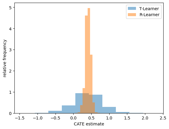
Comparing estimates

We can now compare the CATE estimates produced by both MetaLearners on a histogram:

import matplotlib.pyplot as plt

fig, ax = plt.subplots()

ax.hist(simplify_output(cate_estimates_tlearner), density=True, alpha=.5, label="T-Learner")
ax.hist(simplify_output(cate_estimates_rlearner), density=True, alpha=.5, label="R-Learner")
ax.legend()
ax.set_xlabel("CATE estimate")
ax.set_ylabel("relative frequency")
plt.show()